Flow on the Go
Fast, accurate optical flows on mobile GPUs.
Final Results (Updated May 12th, 2017)
Ashwin Sekar (asekar) and Richard Zhao (richardz)
Summary
We implement realtime, high resolution optical flows on a mobile GPU platform. Fast optical flows allow a realtime video processing pipeline to use the flow in other algorithms such as object detection or image stabilization.
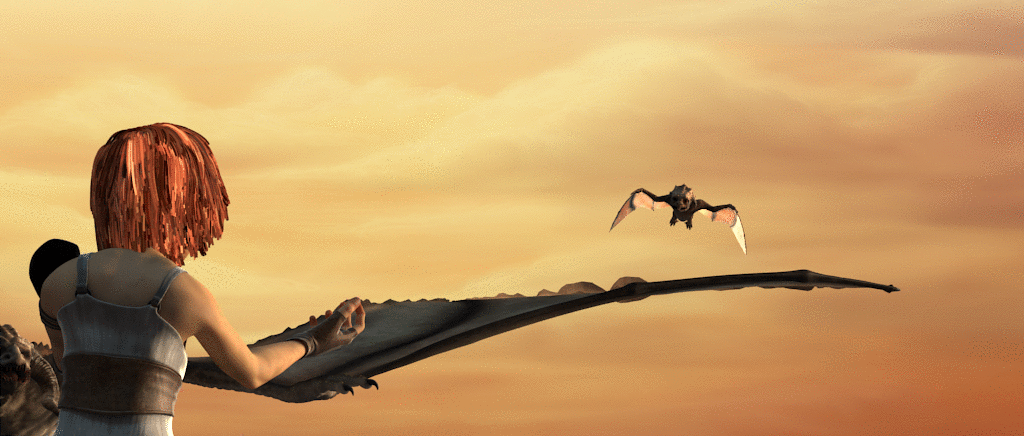

The top gif is an input frame sequence, from which we calculate an optical flow (bottom) which represents movement of subjects in the input.
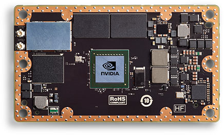
We achieve a speedup of 3x over an optimized CPU baseline on the NVIDIA Jetson TX2 (pictured below), allowing realtime optical flow computation of high resolution video footage (1024 x 448) at 25 frames per second on embedded systems such as drones and autonomous vehicles.
Background
Challenges
The main technical challenges associated with this project involve optimizing the algorithm to run on the NVIDIA Jetson, which has a less powerful CPU and GPU than traditional desktop machines. In particular, the GPU unit on the Jetson has just 2 streaming multiprocessors, compared to 20 on the desktop GTX 1080’s. Additionally, the Jetson has a TDP of just 7.5W, compared to 180W on the GTX 1080.
Since copying memory between the device and host is the main performance bottleneck, we designed the architecture as a pipeline which essentially performs copies at just the beginning and end of the pipeline.
The most significant computational bottleneck in the original implementation was the construction of image pyramids (a series of downsampled images, and their gradients). We used CUDA kernels to significantly improve the performance of this step.
Additionally, during the gradient descent phase of the algorithm, which acts on local patches of the image, careful management of thread blocks is required to hide the system’s memory latency.
Finally, all of our optimizations are done while preserving the accuracy of the computed flow. This makes our approach both fast and accurate enough for realtime use.
Approach
We implemented an Inverse Lucas Kanade approach. When given two frames we constructed image pyramids containing the padded image as well as it’s gradients at different levels. From there we found the optical flow at the coarsest level (smallest image scale), and walked down the pyramid to refine our flow.
To actually find the optical flow at each level, we created a grid of overlapping patches over the image. For each patch we sampled the image as well as the gradients. Using the gradients we were able to compute the Hessian matrix for each patch. From there we initialized the flow for the midpoints of each patch as the upsampled flow from the previous pyramid level (or 0 if this was the first level). We then performed gradient descent iterations to find the true flow for the midpoints.
The gradient descent involved finding the patch in the next frame that this patch mapped to based on the flow. After interpolating this new patch (as the flow is on a real scale, not necessarily integers), we computed the cost function to assess how good our flow performed. The cost function we choose for this task was the L2 norm. With this cost function we were able to calculate the direction of steepest descent and update our flow accordingly. We tuned our convergence parameters to balance accuracy as well as speed.
After the flows for the midpoints were calculated using gradient descent we used densification to extrapolate the flows for the rest of the patch. Specifically, for each pixel of the image we looked at which patches it was a part of, and the accuracy of the flow for that pixel using each patch. From there we were able to assign weights to each patch and took a weighted average of the flows to find the true flow of the pixel.
After this we had a fast and reasonably accurate flow image. In order to improve accuracy even further we applied an additional variational refinement step. Specifically we computed smoothness and gradient data terms for the flow image. We wanted to maximize smoothness and accuracy of our gradients so we tried to minimize this term. This involfved computing various integrals describing the mathematical properties of the flow. From this we were able to create a system of equations that described this minimization. The last step was performing successive-over-relaxation to find an approximate solution for this system of equations and adjust the flow accordingly. This step was by far the hardest to parallelize as it was not inherently data parallel, but contributed to the most accuracy gains.
For implementation we coded three algorithms. Firstly we created a cpu baseline which translated the above description into code, and then multithreaded over all the patches during gradient descent. In all of the involved math operations (Computing the loss function, extrapolating the patch, variational refinement) we implemented vector instructions to achieve even more speedup.
The second implementation converted our data to the GPU and used cuBLAS (a cuda linear algebra library) to perform all mathematical calculations. (Matrix multiplication, gradients, hessian computation, loss function as well as calculations for SOR).
Dismayed with the performance of cuBLAS we created another implementation that used custom THRUST functions to accomplish the mathematical calculations.
Finally, unimpressed with the preformance of the two out of box implementations, we created a custom CUDA implementation. With this approach we were able to parallelize over all patches, and perform 32 wide SIMD on the Jeston to speedup computation within each patch. We were able to control data access patterns to maximize cache use. We were able to control our blocking as well as our memory use for even larger speedup. By using custom filters for the image pyramid construction, we were able to perform all involved calculations on the GPU which contributed greatly to our speedup.
Results
We test on two hardware platforms at two resolutions. For hardware we used
- GHC Machines: Intel Xeon e5 (16 logical cores), NVIDIA GTX 1080 (2560 CUDA cores)
- Jetson TX2: ARM A57 (4 logical cores), 256 CUDA cores
and tested at two resolutions:
- 1024 x 448
- 3840 x 2160 (i.e. 4K)
Accuracy
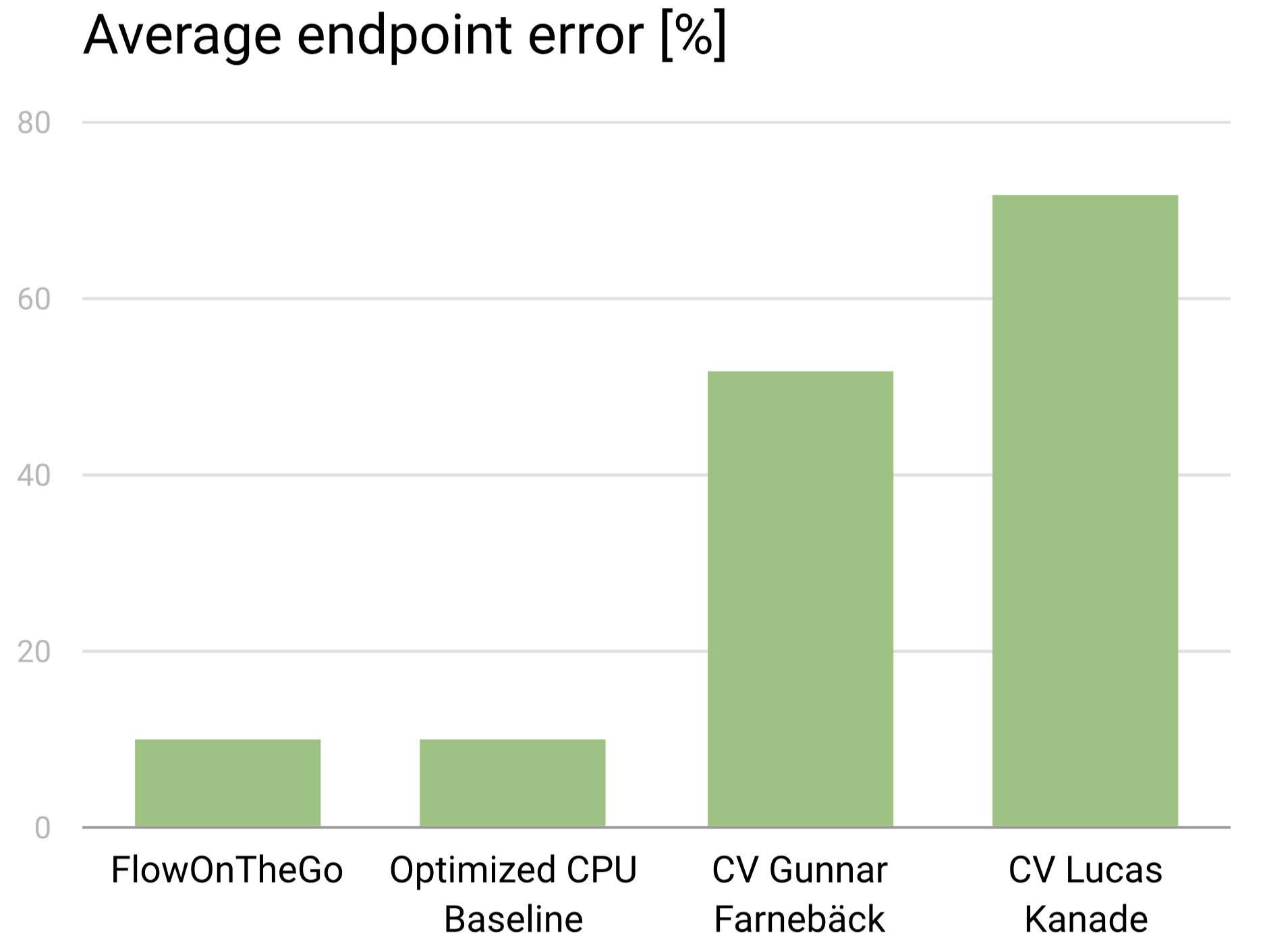
We find that we are able to completely preserve the accuracy of the optical flow as we moved from the optimized CPU baseline to our GPU implementation. Above is a chart (lower is better) of the average endpoint error in our implemenation, which describes the normalized error in the magnitude of direction of the entire flow compared to a ground truth (we used training images from the MPI Sintel dataset, which provides exact ground truths).
On the far left is our implementation, which we compare to the CPU baseline and two common OpenCV implementations.
The biggest gains in accuracy the we had were due to the Variational Refinement. Because we perform smoothing as well as densification we are able to outperform common algorithms such as Lucas Kanade and Gunnar Farneback. The trade off however is speed. We had to optimize heavily to achieve the performance we wanted while maintaining this high level of accuracy.
For comparison the best Optical Flow solvers in existence are Deep Neural Networks which achieve around 5-7% endpoint error, making our implementation very competitive. It is also important to note that test implemenations take in the order of seconds (and sometimes minutes) to evaluate, whereas our approach (~10% endpoint error) runs in realtime.
Optical Flow Runtimes
We now present the results of our project.
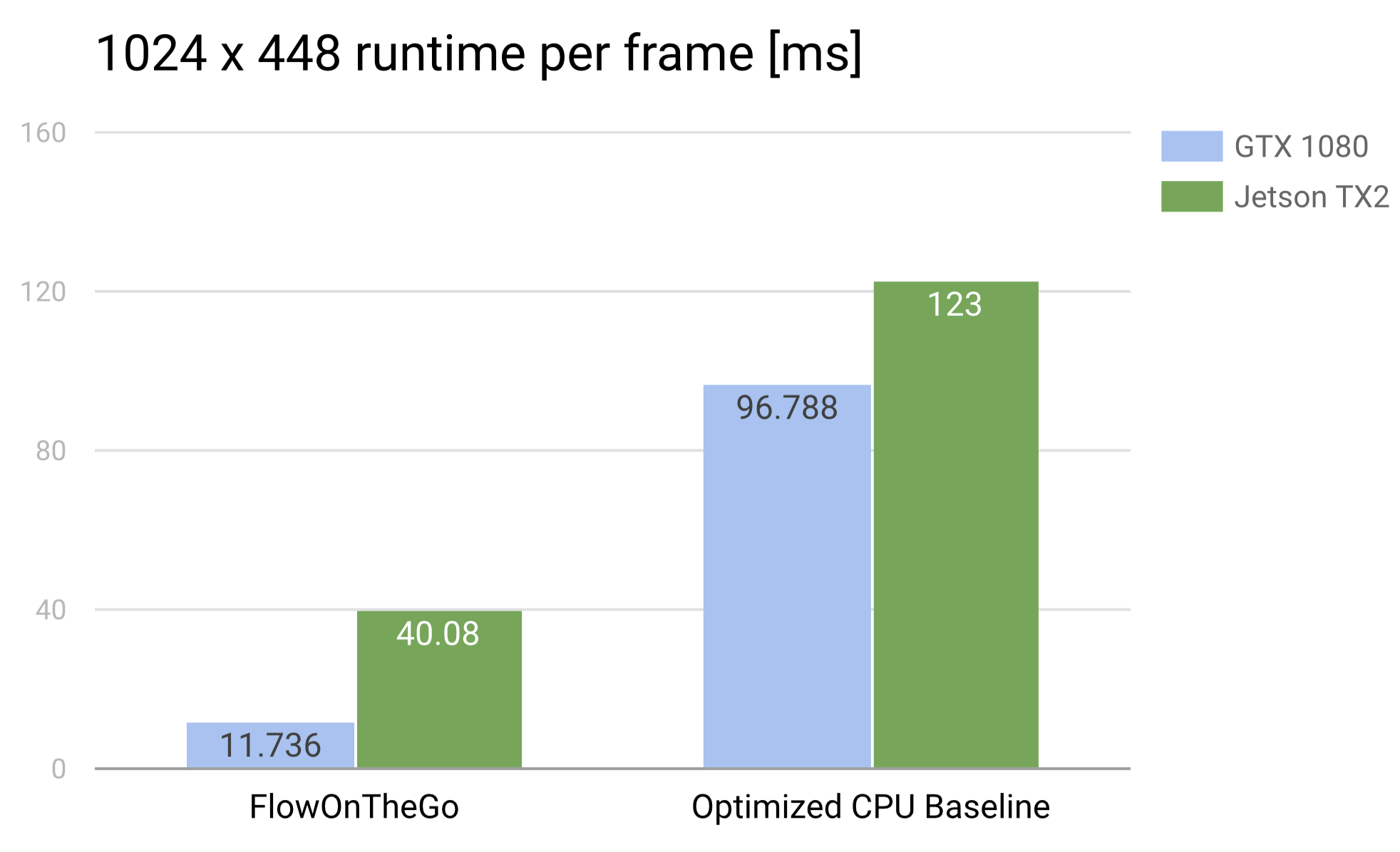
1024 x 448
Above is a chart of average runtimes achieved by Flow on the Go and our optimized CPU benchmark for 1024x448 resolution images on both types of hardware.
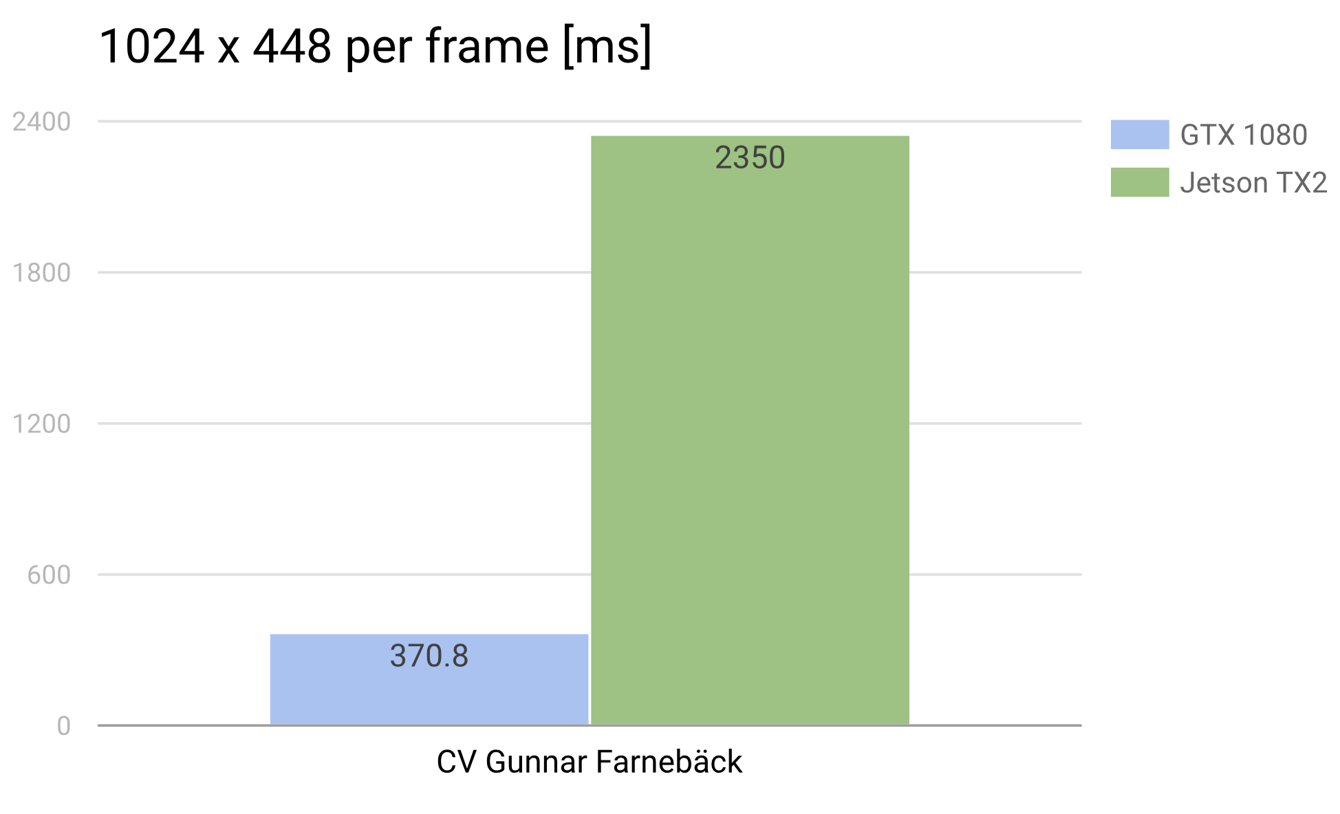
Below is a chart comparing OpenCV’s CPU optical flow implementation on the GHC machines verus on the Jetson. It was excluded from the above chart since its runtime is several orders of magnitude higher.
3840 x 2160
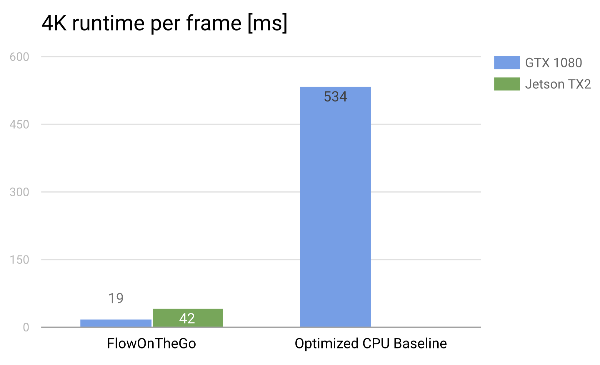
Above is a chart of average runtimes achieved by Flow on the Go and the optimized CPU benchmark on 4K resolution images. The speedup achieved by our implementation dramatically increases with the image size, which makes sense as GPU’s are better at scaling up due to parallel workload. The Jetson is able to process a single frame in roughly 40 milliseconds, enabling it to process a 4K resolution video in realtime at 25 frames per second.
Processing a single 4K image using an OpenCV CPU implementation takes roughly 50,000 ms (1250x slower) on the Jetson and 8000 ms (420x slower) on the GHC machines.
References
The approach is entirely based on the work of
Tim Kroeger, et. al Fast Optical Flow using Dense Inverse Search (2016)
and the codebase accompanying the publication.
The colorization and accuracy evaluation were done using the methodology and tools created by
A Database and Evaluation Methodology for Optical Flow, International Journal of Computer Vision, 92(1):1-31, March 2011.
which can be found here.
Work Division
Aside from specific tasks listed below, all work was done together.
Richard
- Background research and project selection
- Image pyramid construction
- Variational refinement kernels
Ashwin
- Patch extration (3 implementations)
- Gradient descent
- Aggregate densification
- Memory pipeline